Riemann Zeta Function Zeros

Zeros of the Riemann zeta function come in two different types. So-called "trivial zeros" occur at all negative even integers , , , ..., and "nontrivial zeros" occur at certain values of satisfying

(1)

for in the "critical strip" . In general, a nontrivial zero of is denoted , and the th nontrivial zero with is commonly denoted (Brent 1979; Edwards 2001, p. 43), with the corresponding value of being called .

Wiener (1951) showed that the prime number theorem is literally equivalent to the assertion that has no zeros on (Hardy 1999, p. 34; Havil 2003, p. 195). The Riemann hypothesis asserts that the nontrivial zeros of all have real part , a line called the "critical line." This is known to be true for the first zeros.

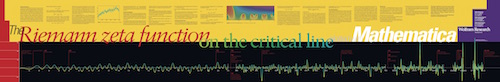
An attractive poster plotting zeros of the Riemann zeta function on the critical line together with annotations for relevant historical information, illustrated above, was created by Wolfram Research (1995).

Min Max Re Im

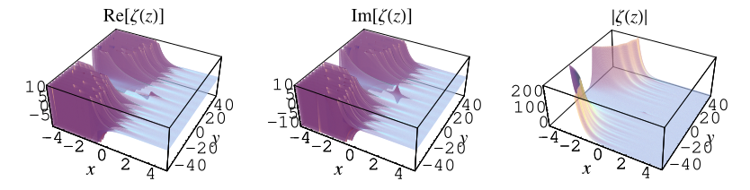
The plots above show the real and imaginary parts of plotted in the complex plane together with the complex modulus of . As can be seen, in right half-plane, the function is fairly flat, but with a large number of horizontal ridges. It is precisely along these ridges that the nontrivial zeros of lie.

The position of the complex zeros can be seen slightly more easily by plotting the contours of zero real (red) and imaginary (blue) parts, as illustrated above. The zeros (indicated as black dots) occur where the curves intersect.

The figures above highlight the zeros in the complex plane by plotting (where the zeros are dips) and (where the zeros are peaks).

The above plot shows for between 0 and 60. As can be seen, the first few nontrivial zeros occur at the values given in the following table (Wagon 1991, pp. 361-362 and 367-368; Havil 2003, p. 196; Odlyzko), where the corresponding negative values are also roots. The integers closest to these values are 14, 21, 25, 30, 33, 38, 41, 43, 48, 50, ... (OEIS A002410). The numbers of nontrivial zeros less than 10, , , ... are 0, 29, 649, 10142, 138069, 1747146, ... (OEIS A072080; Odlyzko).

	OEIS
1	A058303	14.134725
2		21.022040
3		25.010858
4		30.424876
5		32.935062
6		37.586178

The so-called xi-function defined by Riemann has precisely the same zeros as the nontrivial zeros of with the additional benefit that is entire and is purely real and so are simpler to locate.

ZetaGrid is a distributed computing project attempting to calculate as many zeros as possible. It had reached 1029.9 billion zeros as of Feb. 18, 2005. Gourdon (2004) used an algorithm of Odlyzko and Schönhage to calculate the first zeros (Pegg 2004, Pegg and Weisstein 2004). The following table lists historical benchmarks in the number of computed zeros (Gourdon 2004).

year		author
1903	15	J. P. Gram
1914	79	R. J. Backlund
1925	138	J. I. Hutchinson
1935		E. C. Titchmarsh
1953		A. M. Turing
1956		D. H. Lehmer
1956		D. H. Lehmer
1958		N. A. Meller
1966		R. S. Lehman
1968		J. B. Rosser, J. M. Yohe, L. Schoenfeld
1977		R. P. Brent
1979		R. P. Brent
1982		R. P. Brent, J. van de Lune, H. J. J. te Riele, D. T. Winter
1983		J. van de Lune, H. J. J. te Riele
1986		J. van de Lune, H. J. J. te Riele, D. T. Winter
2001		J. van de Lune (unpublished)
2004		S. Wedeniwski
2004		X. Gourdon and P. Demichel

Numerical evidence suggests that all values of corresponding to nontrivial zeros are irrational (e.g., Havil 2003, p. 195; Derbyshire 2004, p. 384).

No known zeros with order greater than one are known. While the existence of such zeros would not disprove the Riemann hypothesis, it would cause serious problems for many current computational techniques (Derbyshire 2004, p. 385).

Some nontrivial zeros lie extremely close together, a property known as Lehmer's phenomenon.

The Riemann zeta function can be factored over its nontrivial zeros as the Hadamard product

(2)

(Titchmarsh 1987, Voros 1987).

Let denote the th nontrivial zero of , and write the sums of the negative integer powers of such zeros as

(3)

(Lehmer 1988, Keiper 1992, Finch 2003, p. 168), sometimes also denoted (e.g., Finch 2003, p. 168). But by the functional equation, the nontrivial zeros are paired as and , so if the zeros with positive imaginary part are written as , then the sums become

(4)

Such sums can be computed analytically, and the first few are

			(5)
			(6)
			(7)
			(8)
			(9)
			(10)

where is the Euler-Mascheroni constant, are Stieltjes constants, is the Riemann zeta function, and is Apéry's constant. These values can also be written in terms of the Li constants (Bombieri and Lagarias 1999).

The case

(11)

(OEIS A074760; Edwards 2001, p. 160) is classical and was known to Riemann, who used it in his computation of the roots of (Davenport 1980, pp. 83-84; Edwards 2001, pp. 67 and 159). It is also equal to the constant from Li's criterion.

Assuming the truth of the Riemann hypothesis (so that ), equation (◇) can be written for the first few values of in the simple forms

			(12)
			(13)
			(14)
			(15)

and so on.