Polynomial Roots

A root of a polynomial is a number such that . The fundamental theorem of algebra states that a polynomial of degree has roots, some of which may be degenerate. For example, the roots of the polynomial

(1)

are , 1, and 2. Finding roots of a polynomial is therefore equivalent to polynomial factorization into factors of degree 1.

Any polynomial can be numerically factored, although different algorithms have different strengths and weaknesses.

The roots of a polynomial equation may be found exactly in the Wolfram Language using Roots[lhs==rhs, var], or numerically using NRoots[lhs==rhs, var]. In general, a given root of a polynomial is represented as Root[#^n+a[n-1]#^(n-1)+...+a[0]&, k], where , 2, ..., is an index identifying the particular root and the pure function polynomial is irreducible. Note that in the Wolfram Language, the ordering of roots is different in each of the commands Roots, NRoots, and Table[Root[p, k], k, n].

In the Wolfram Language, algebraic expressions involving Root objects can be combined into a new Root object using the command RootReduce.

In this work, the th root of a polynomial in the ordering of the Wolfram Language's Root object is denoted , where is a dummy variable. In this ordering, real roots come before complex ones and complex conjugate pairs of roots are adjacent. For example,

			(2)
			(3)

and

			(4)
			(5)
			(6)

Let the roots of the polynomial

(7)

be denoted , , ..., . Then Vieta's formulas give

			(8)
			(9)
			(10)

These can be derived by writing

(11)

expanding, and then comparing the coefficients with (◇).

Given an th degree polynomial , the roots can be found by finding the eigenvalues of the matrix

(12)

and taking . This method can be computationally expensive, but is fairly robust at finding close and multiple roots.

If the coefficients of the polynomial

(13)

are specified to be integers, then rational roots must have a numerator which is a factor of and a denominator which is a factor of (with either sign possible). This is known as the polynomial remainder theorem.

If there are no negative roots of a polynomial (as can be determined by Descartes' sign rule), then the greatest lower bound is 0. Otherwise, write out the coefficients, let , and compute the next line. Now, if any coefficients are 0, set them to minus the sign of the next higher coefficient, starting with the second highest order coefficient. If all the signs alternate, is the greatest lower bound. If not, then subtract 1 from , and compute another line. For example, consider the polynomial

(14)

Performing the above algorithm then gives

0	2	2		1
	2	0		8
--	2			8
	2			7
	2		5		35

so the greatest lower bound is .

If there are no positive roots of a polynomial (as can be determined by Descartes' sign rule), the least upper bound is 0. Otherwise, write out the coefficients of the polynomials, including zeros as necessary. Let . On the line below, write the highest order coefficient. Starting with the second-highest coefficient, add times the number just written to the original second coefficient, and write it below the second coefficient. Continue through order zero. If all the coefficients are nonnegative, the least upper bound is . If not, add one to and repeat the process again. For example, take the polynomial

(15)

Performing the above algorithm gives

0	2			1
1	2	1
2	2	3
3	2	5	8	25	68

so the least upper bound is 3.

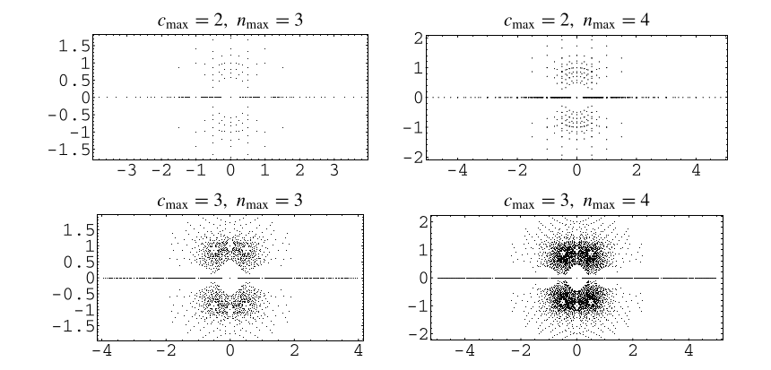
Plotting the roots in the complex plane of all polynomials up to some degree with integer coefficients less than some cutoff integer in absolute value shows the beautiful structure illustrated above (Trott 2004, p. 23).

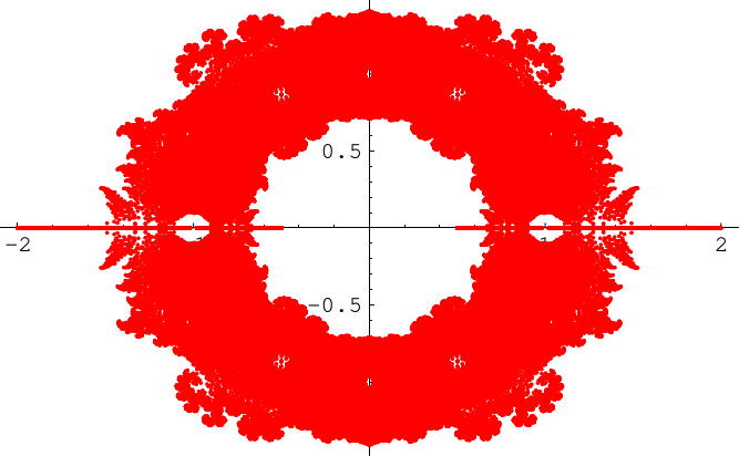
An even more stunning figure is obtained by plotting all roots of all polynomials with coefficients up to degree (Borwein and Jörgenson 2001; Pickover 2002; Bailey et al. 2007, p. 18).