A convolution is an integral that expresses the amount of overlap of one function as it is shifted over another function
. It therefore "blends" one
function with another. For example, in synthesis imaging, the measured dirty map
is a convolution of the "true" CLEAN map with the dirty beam (the Fourier
transform of the sampling distribution). The convolution is sometimes also known
by its German name, faltung ("folding").
Convolution is implemented in the Wolfram Language as Convolve[f, g, x, y] and DiscreteConvolve[f, g, n, m].
Abstractly, a convolution is defined as a product of functions and
that are objects in the algebra of Schwartz functions
in
. Convolution of two functions
and
over a finite range
is given by
|
(1)
|
where the symbol
denotes convolution of
and
.
Convolution is more often taken over an infinite range,
|
(2)
| |||
|
(3)
|
(Bracewell 1965, p. 25) with the variable (in this case ) implied, and also occasionally written as
.

|

|
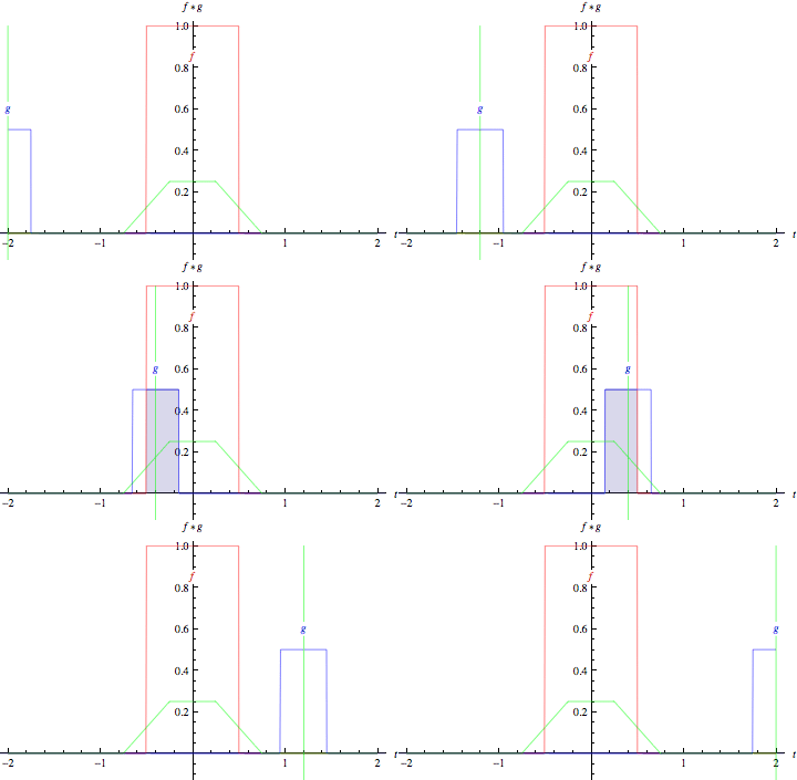
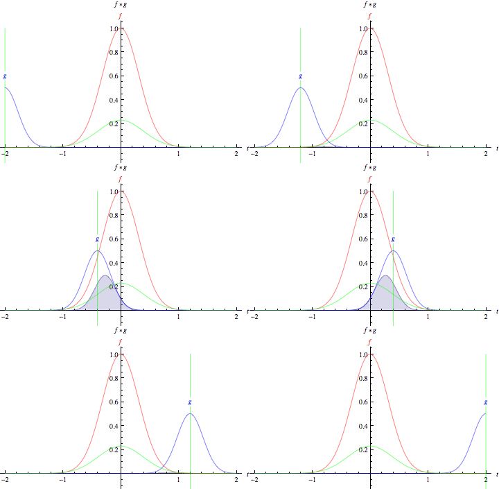
The animations above graphically illustrate the convolution of two boxcar functions (left) and two Gaussians (right).
In the plots, the green curve shows the convolution of the blue and red curves as
a function of ,
the position indicated by the vertical green line. The gray region indicates the
product
as a function of
,
so its area as a function of
is precisely the convolution. One feature to emphasize and
which is not conveyed by these illustrations (since they both exclusively involve
symmetric functions) is that the function
must be mirrored before lagging it across
and integrating.
The convolution of two boxcar functions and
has the particularly simple form
![f*g=[(t-t_1-u_1)H(t-t_1-u_1)-(t-t_2-u_1)H(t-t_2-u_1)
-(t-t_1-u_2)H(t-t_1-u_2)+(t-t_2-u_2)H(t-t_2-u_2)],](/images/equations/Convolution/NumberedEquation2.svg) |
(4)
|
where
is the Heaviside step function. Even more
amazingly, the convolution of two Gaussians
|
(5)
| |||
|
(6)
|
is another Gaussian
![f*g=1/(sqrt(2pi(sigma_1^2+sigma_2^2)))e^(-[t-(mu_1+mu_2)]^2/[2(sigma_1^2+sigma_2^2)]).](/images/equations/Convolution/NumberedEquation3.svg) |
(7)
|
Let ,
, and
be arbitrary functions and
a constant. Convolution satisfies the properties
|
(8)
| |||
|
(9)
| |||
|
(10)
|
(Bracewell 1965, p. 27), as well as
|
(11)
| |||
|
(12)
|
(Bracewell 1965, p. 49).
Taking the derivative of a convolution gives
|
(13)
| |||
|
(14)
|
(Bracewell 1965, p. 119).
The area under a convolution is the product of areas under the factors,
|
(15)
| |||
|
(16)
| |||
|
(17)
|
The horizontal function centroids of a convolution add
|
(18)
|
and provided that either
or
has its function
centroids at its origin, the variances do as well
|
(19)
|
(Bracewell 1965, p. 142), where
 |
(20)
|
There is also a definition of the convolution which arises in probability theory and is given by
|
(21)
|
where
is a Stieltjes integral.